


Chapter 8: DC-DC Converters
8.1: Introduction
The topics covered in this chapter are as follows:
- Classification of converters.
- Principle of Step Down Operation.
- Buck Converter with R-L-E Load.
- Buck Converter with R Load and Filter.
8.2: Classification of Converters
The converter topologies are classified as:
- Buck Converter: In figure 8.1a
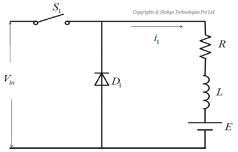
Figure 8.1a: General configuration of buck converter., a buck converter is shown. The buck converter is step down converter and produces a lower average output voltage than the DC input voltage. - Boost converter: In figure 8.1b
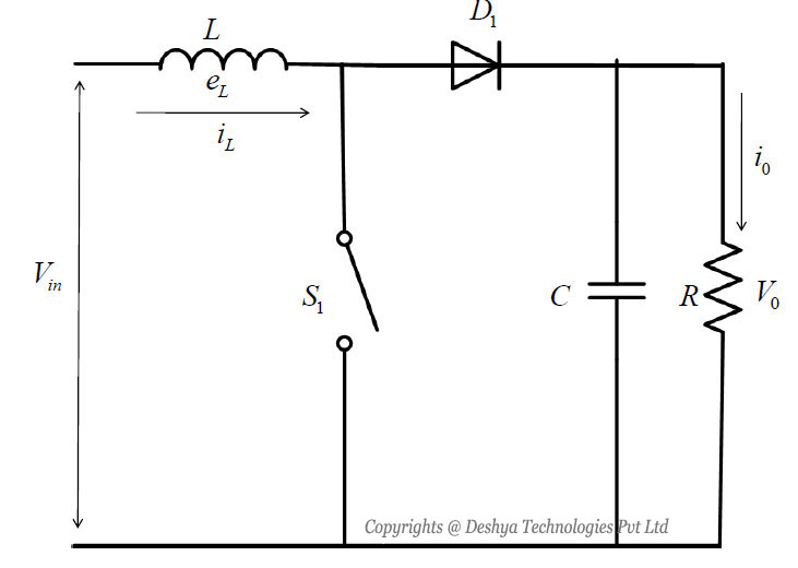
Figure 8.1b:General Configuration Boost Converter., a boost converter is shown. The output voltage is always greater than the input voltage. - Buck-Boost converter: In figure 8.1c
Figure 8.1c: General Configuration Buck-Boost Converter., a buck-boost converter is shown. The output voltage can be either higher or lower than the input voltage.
Figure 8.1a: General Configuration Buck Converter.
Figure 8.1b: General Configuration Boost Converter.
Figure 8.1c: General Configuration Buck-Boost Converter.
8.3: Principle of step down operation
The principle of step down operation of DC-DC converter is explained using the circuit shown in figure 8.2a 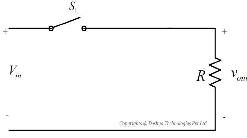
Figure 8.2a: Step down operation.. When the switch S1 is closed for time duration T1, the input voltage Vin appears across the load. For the time duration T2 switch S1 remains open and the voltage across the load is zero. The waveforms of the output voltage across the load are shown in figure 8.2b 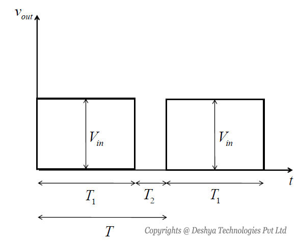
Figure 8.2b: Voltage across the load resistance.
Figure 8.2a: Step down operation.
Figure 8.2b: Voltage across the load resistance.
The average output voltage is given by
 |
(8.1) |
The average load current is given by
 |
(8.2) |
where
T is the chopping period
 is the duty cycle
f is the chopping frequency
The rms value of the output voltage is given by
 |
(8.3) |
In case the converter is assumed to be lossless, the input power to the converter will be equal to the output power. Hence, the input power (Pin) is given by
 |
(8.4) |
The effective resistance seen by the source is (using equation 8.2
)
 |
(8.5) |
The duty cycle D can be varied from 0 to 1 by varying T1, T or f. Thus, the output voltage Voavg can be varied from 0 to Vin by controlling D and eventually the power flow can be controlled.
8.4: The Buck Converter with R-L-E Load
A buck converter with R-L-E load is shown in figure 8.3 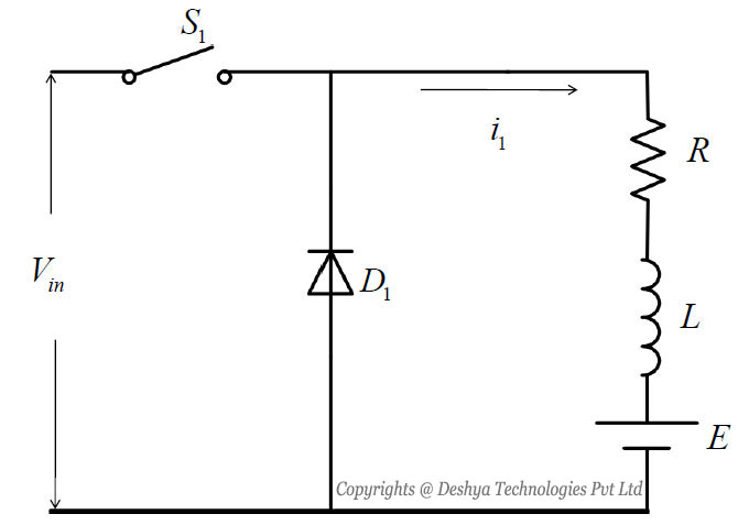
Figure 8.3: Schematics of a buck converter feeding a R-L-E load..
Figure 8.3: Schematics of a buck converter feeding a R-L-E load.
The buck converter is a voltage step down and current step up converter. The two modes in steady state operations are:
Mode 1 Operation
In this mode the switch S1 is turned on and the diode D1 is reversed biased, the current flows through the load. The time domain circuit is shown in figure 8.4a 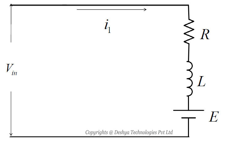
Figure 8.4a: Time domain circuit of buck converter in mode 1.. The load current, in s domain, for mode 1 can be found from
 |
(8.6) |
Where
I01 is the initial value of the current and I01=I1
Figure 8.4a: Time domain circuit of buck converter in mode 1.
From equation 8.6
, the current i1(s) is given by
 |
(8.7) |
In time domain the solution of equation 8.7
is given by
 |
(8.8) |
The mode 1 is valid for the time duration 0 ≤ t ≤ T1 Þ 0 ≤ t ≤ DT . At the end of this mode, the load current becomes
 |
(8.9) |
Mode 2 Operation
In this mode the switch S1 is turned off and the diode D1 is forward biased. The time domain circuit is shown in figure 8.4b 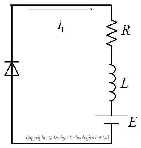
Figure 8.4b: Time domain circuit of buck converter in mode 2.. The load current, in domain, can be found from
 |
(8.10) |
Where
I02 is the initial value of the load current
The current at the end of mode 1 is equal to the current at the beginning of mode 2. Hence, from equation 8.9
T02 is obtained as
 |
(8.11) |
Figure 8.4b: Time domain circuit of buck converter in mode 2.
Hence, the load current in time domain is obtained from equation 8.10
as
 |
(8.12) |
The equation 8.12
is valid for the time duration DT ≤ t ≤ T
Determination of I1 and I2
At the end of mode 2 the load current becomes
 |
(8.13) |
At the end of mode 2, the converter enters mode 1 again. Hence, the initial value of current in
 |
(8.14) |
From equation 8.8
and equation 8.12
the following relation between I1 and I2 is obtained as
 |
(8.15) |
 |
(8.16) |
Solving equation 8.15
and equation 8.16
for I1 and I2 gives
 |
(8.17) |
 |
(8.18) |
Where
 |
(8.19) |
where f is the chopping frequency.
The load current waveform for a buck converter with R-L-E load is shown in figure 8.5 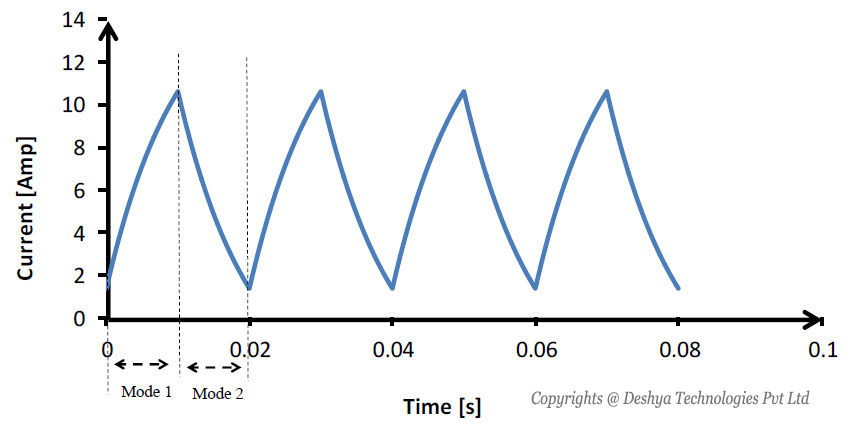
Figure 8.5: Current through R-L-E load..
Figure 8.5: Current through R - L - E load.
The operation of the buck converter with R-L-E load is shown in Animation 8.1
\Animation 8.1: Buck converter for continouse conduction.
Current Ripple
The peak to peak current ripple is given by
 |
(8.20) |
To determine the current the maximum current ripple (∆Imax), the equation 8.20
is differentiated w.r.t D. This give
 |
(8.21) |
The duty ratio (Dmax) at which maximum current ripple occurs is given by setting equation 8.21
equal to zero, i.e.
 |
(8.22) |
Substituting the value of Dmax=0.5 in equation 8.20
gives the maximum current ripple (∆Imax) as
 |
(8.23) |
For the condition 4fL >> R,
 |
(8.24) |
Hence the maximum current ripple is given by
 |
(8.25) |
From equation 8.20
the normalized peak to peak ripple current (∆I) is given by
 |
(8.26) |
In figure 8.6 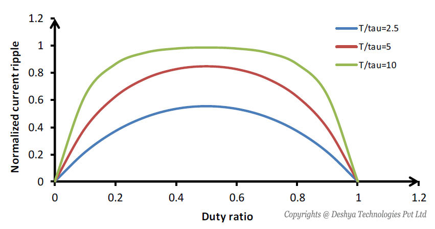
figure 8.6: Normalized current ripple versus duty ratio. the duty ratio versus normalized current ripple (∆Inormalized) curve is shown by
Figure 8.6: Normalized current ripple versus duty ratio.
From figure 8.6
figure 8.6: Normalized current ripple versus duty ratio. the following conclusions can be drawn
- The ripple current reduces to zero as D → 0 and D → 1 .
- The maximum ripple current occurs at D = 0 .
From figure 8.7 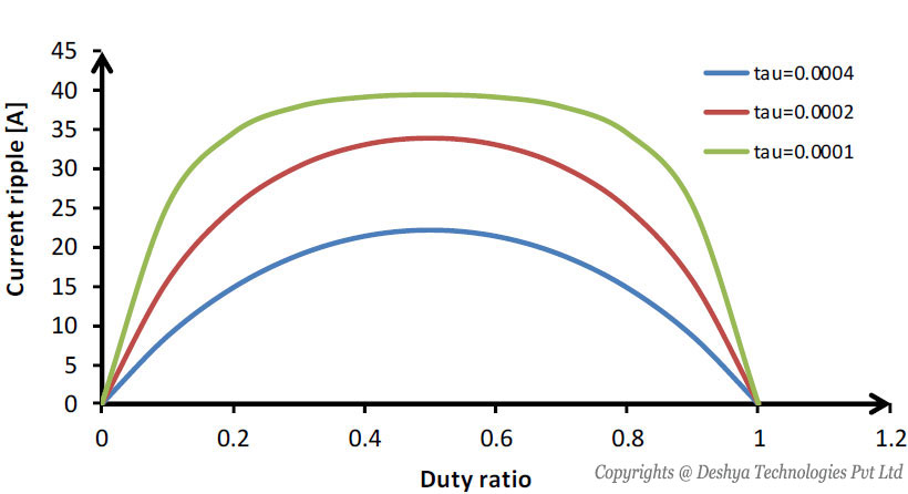
figure 8.7: Current ripple versus duty ratio for a fixed switching frequency., the ripple current (∆I) versus duty ratio for different values of time constant ( ) is shown. The time constant is varied by changing the values inductance (L)
Figure 8.7: Current ripple versus duty ratio for a fixed switching frequency.
From figure 8.7
Figure 8.7: General configuration of buck converter., it can be seen that, as time constant increases (keeping the resistance constant and increasing the inductance), the magnitude of the current ripple increases. In figure 8.8 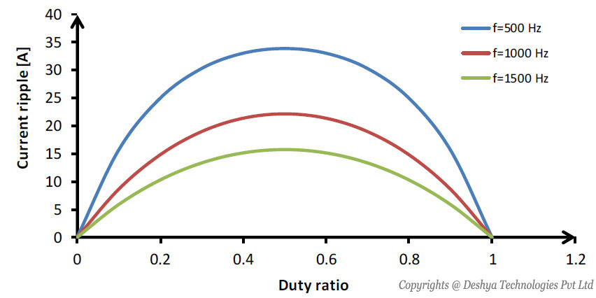
Figure 8.8: General configuration of buck converter., the current ripple versus duty ratio for different switching frequency (keeping the resistance and inductance constant) is shown. From figure 8.8
Figure 8.8: General configuration of buck converter., it can be seen that as the switching frequency increases, the current ripple decreases. Hence, from equation 8.20
, figure 8.6
Figure 8.6: Normalized current ripple versus duty ratio., figure 8.7
Figure 8.7: General configuration of buck converter. and figure 8.8
Figure 8.8: Current ripple versus duty ratio for varying switching frequency. the following conclusions can be drawn:
- The current ripple is independent of load voltage E.
- The ripple current reduces to zero as D → 0 and D → 1 .
- The maximum ripple current occurs at D = 0 .
- As time constant increases (keeping the resistance constant and increasing the inductance), the magnitude of the current ripple increases.
- As the switching frequency increases (keeping the resistance and inductance constant), the current ripple decreases.
Figure 8.8: Current ripple versus duty ratio for a varying switching frequency.
Average and r.m.s values of input and diode currents
In mode 1 operation, the switch S1 is on and the current passes through the switch (figure 8.4a
Figure 8.4a: Time domain circuit of buck converter in mode 1.) and the instantaneous current is given by equation 8.8
. In mode 2, the switch is off and the load current flows through the diode D1 (figure 8.4b
Figure 8.4b: Time domain circuit of buck converter in mode 2.) and the instantaneous current is given by equation 8.12
. Hence, the average load current is given by
 |
(8.27) |
Substituting the values of i1(t) and i2(t) from equation 8.8
and equation 8.12
into equation 8.27
and solving it gives
 |
(8.28) |
In mode 1 the current flows through the switch, hence, the average switch current can be obtained by integrating the instantaneous load current given by equation 8.8
over a time period T, that is
 |
(8.29) |
The currents I1 and I2 are given by equation 8.17
and equation 8.18
. In mode 2 the diode conducts and the instantaneous current is given by equation 8.12
. The average diode current can be obtained by integrating equation 8.12
over a time period, that is
 |
(8.30) |
Fourier series analysis of the output voltage and load current for R-L-E load is given in Box 8.1.
Box 8.1.
The time domain expression of load current in case of a converter with R-L load (figure 8.B1.1 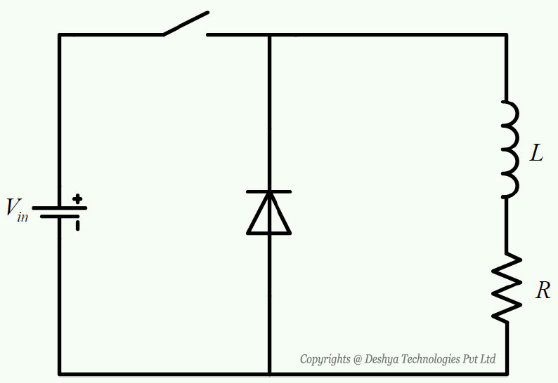
Figure 8.B1.1: Buck converter with R-L load.) can be obtained by setting E=0 in the equation 8.8
and equation 8.12
Figure 8.B1.1: Buck converter with R-L load.
However, it is also possible to obtain the time domain expression of output voltage and load current using the Fourier series. The output voltage of the DC-DC buck converter is shown in figure 8.B1.2 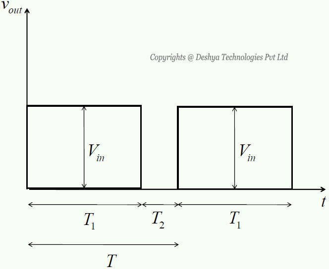
Figure 8.B1.2: Voltage across the load.. From figure 8.B1.2
Figure 8.B1.2: Voltage across the load. it can be seen that the output voltage is a series of rectangular pulses. The Fourier series representation of the pulse train is
 |
(8.B1.1) |
The Fourier coefficients a0, an and bn are given by
 |
(8.B1.2) |
The output voltage (Vout) is given by
 |
(8.B1.3) |
From equation 8.2
, it can be seen that. Hence, equation 8.B1.3
can be written as
 |
(8.B1.4) |
Using equation 8.B1.4
in equation 8.B1.1
gives
 |
(8.B1.5) |
Substituting  in equation 8.B1.5
gives
 |
Substituting the coefficients a0, an and bn into equation 8.B1.1
gives
 |
(8.B1.6) |
The equation 8.B1.6
can be written as
 |
(8.B1.7) |
Simplifying equation 8.B1.7
gives
 |
(8.B1.8) |
Figure 8.B1.2: Voltage across the load.
The load current is given by
 |
(8.B1.9) |
The voltage and current waveforms obtained by equation 8.B1.8
and equation 8.B1.9
are shown in figure 8.B1.3 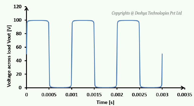
Figure 8.B1.3: Voltage across the load obtaimed from Fourier series representation. and figure 8.B1.4 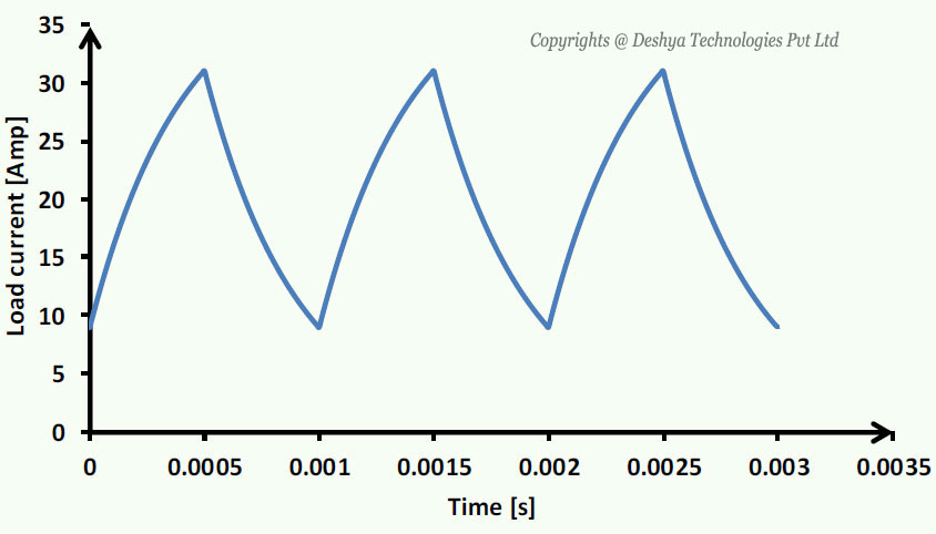
Figure 8.B1.4: Load current obtaimed from Fourier series representation. respectively.
Figure 8.B1.3: Voltage across the load obtained from Fourier series representation.
Figure 8.B1.4: Load current obtained from Fourier series representation.
In case of buck converter with R-L-E (figure 8.B1.5 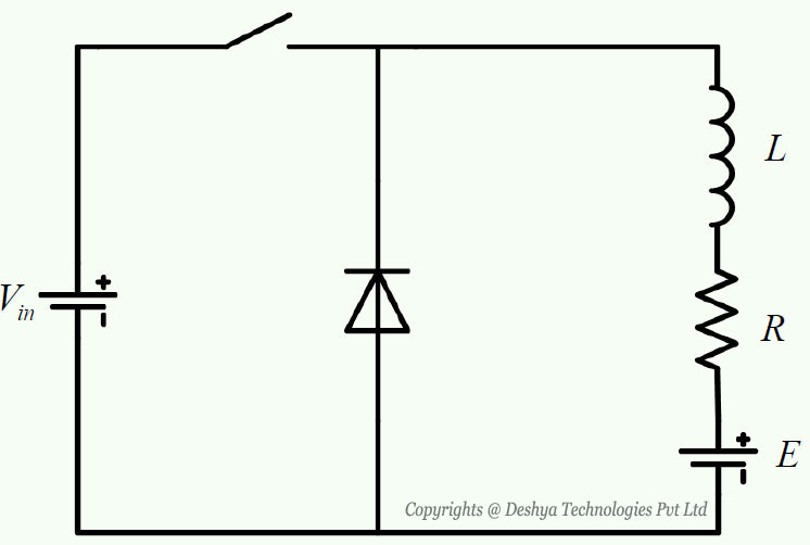
Figure 8.B1.5: Buck converter with R-L-E load.), the voltage across the load is given by equation 8.B1.8
and the current is given by
 |
(8.B1.10) |
The average load current is obtained by integrating equation 8.B1.10
over a time period, that is
 |
(8.B1.11) |
Figure 8.B1.5: Buck converter with R-L-E load.
The analysis of a buck converter is explained in example 8.1.
Example 8.1
A DC-DC buck converter feeds a load that has a resistance of 5 Ω , an inductance of 20mH and an e.m.f. of 50 V DC. The input voltage to the buck converter is 200V DC. The buck converter operates at a frequency of 1kHz and at 50% duty ratio. Determine:
- the load average and r.m.s. voltage.
- the ripple voltage and ripple factor.
- the maximum and minimum output current and the peak to peak output ripple current.
- the current in time domain.
- the average load output current, average switch current and average diode current.
- the input power.
Solution:-
The given parameters of the buck converter are:
Duty ratio (D) = 0.5
The input voltage (Vin) = 200V
The load voltage (E) = 50V
The switching frequency (f) = 1000 Hz
The time period 
The on duration (T1) = DT = 0.5 ms
The off duration (T2) = (1-D)T = 0.5 ms
The load time constant is 
-
load average and load r.m.s voltage
The average load voltage is given by equation 8.1
. Hence,Voavg = DVin = 0.5 x 200 = 10V
The r.m.s value of output voltage is given by equation 8.3

-
ripple voltage and ripple factor
The output AC load voltage is given by
(8.E1.1) Using equation 8.1
and equation 8.3
, the equation 8.E1.1
can be written as
(8.E1.2) Hence

The ripple factor is given by
(8.E1.3) Using equation 8.E1.2
the equation 8.E1.3
can be written as
(8.E1.4) Hence, the ripple factor is
maximum, minimum and peak to peak output ripple current
The minimum output current is given by equation 8.17
The maximum current is given by equation 8.18
The peak to peak output current ripple is given by
∆I = I2 - I1 = 11.25 - 8.75 = 2.5 A
Current in time domain
The switching frequency of the converter is 1000Hz and the time period is

Using equation 8.8
, the current in mode 1 can be written as
and from equation 8.9
in mode 2 is given by
The values of I1 and I2 have been determined in part iii of the solution above
The average load current is given by equation 8.28
as
The average switch current is given by equation 8.29
as
The average diode current is given by
the input power is given by
Pin = Vin x Iswitch = 200 x 5 = 1000 W
Discontinuous Load Current
For a buck converter with R-L-E load it is possible that the load current can reach zero during the period when the switch S1 is off (T1≤ t ≥ T), at a time Tx. The load current thus becomes discontinuous. In figure 8.9 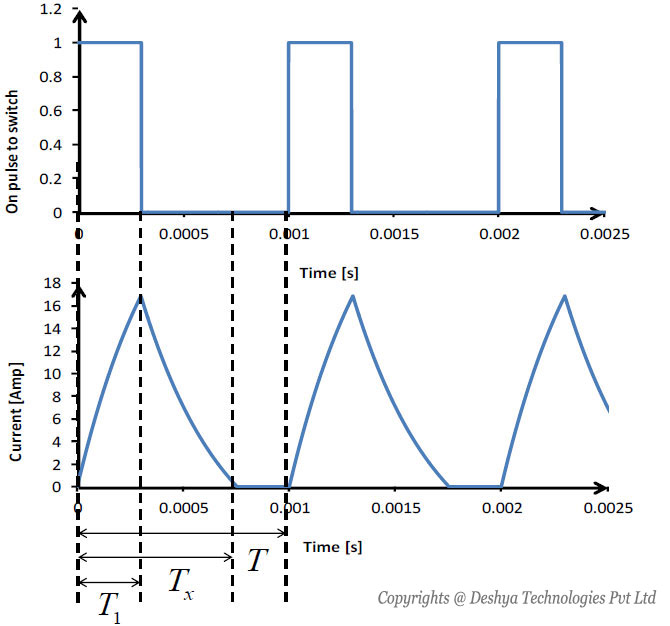
Figure 8.9: Current waveform for buck converter with R-L-E load in discontinous conduction. the discontinuous load current is shown.
Figure 8.9: Current waveform for buck converter with R-L-E load in discontinous conduction.
From figure 8.9
Figure 8.9: General configuration of buck converter. it can be seen that the current through the load becomes zero before the mode 2 ends. The instantaneous current for mode 1 (when the switch S1) is on is given by equation 8.8
. However, in mode 1 the current starts from zero (that is I1=0) and the instantaneous current can be written as
 |
(8.31) |
In mode 2 the instantaneous load current is given by equation 8.12
. However, unlike the continuous conduction scenario, in discontinuous conduction the current exists only up to time instant Tx. Hence, the current in discontinuous conduction mode can be written as,
 |
(8.32) |
To determine I2 we use the following condition
 |
(8.33) |
From equation 8.33
, I2 is obtained as
 |
(8.34) |
The time instant at which the load current becomes zero (Tx) can be obtained by substituting t =Tx in equation 8.32
, that is
 |
(8.35) |
Solving equation 8.35
for Tx gives
 |
(8.36) |
The load voltage for discontinuous conduction is given by
 |
(8.37) |
The load voltage is shown in figure 8.10 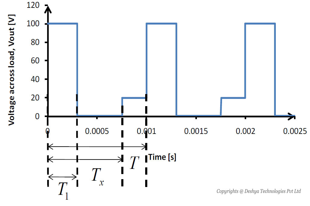
Figure 8.10: Voltage across the load in a buck converter with R-L-E load in case of discontinuous conduction..
Figure 8.10: Voltage across the load in a buck converter with R - L - E load in case of discontinuous conduction.
The average value of voltage across the load is given by
 |
(8.38) |
The r.m.s value of voltage across the load is given by
 |
(8.39) |
The current ripple in case of discontinuous mode of conduction is given by
 |
(8.40) |
In case of discontinuous mode of conduction I1 = 0 and substituting for I2 from equation 8.34
into equation 8.40
gives
 |
(8.41) |
The average load current is given by
 |
(8.42) |
Substituting I1 = 0 and I2 from equation 8.34
into equation 8.41
gives
 |
(8.43) |
Substituting for Vout from equation 8.38
into equation 8.43
gives
 |
(8.44) |
In mode 1 the switch (S1) conducts, hence the average switch current is given by
 |
(8.45) |
In mode 2 the diode conducts for an interval T1≤ t ≤ Tx , hence the average diode current is given by
 |
(8.46) |
The operation of buck converter in discontinuous mode is shown in Animation 8.2. The Fourier analysis of the load voltage and current is given in Box 8.2.
Animation 8.2: Buck converter with discontinuous load current.
Box 8.2
The output voltage of the DC-DC buck converter for discontinuous conduction is shown in figure 8.10
Figure 8.10: Voltage across the load in a buck converter with R-L-E load in case of discontinuous conduction.. From figure 8.10
Figure 8.10: Voltage across the load in a buck converter with R-L-E load in case of discontinuous conduction. it can be seen that the output voltage is a series of rectangular pulses. The Fourier series representation of the pulse train is
 |
(8.B2.1) |
The Fourier coefficients a0, an and bn are given by
 |
(8.B2.2) |
The output voltage (Vout ) is given by
 |
(8.B2.3) |
From equation 8.2
, it can be seen that . Hence, equation 8.B2.3
can be written as
 |
(8.B2.4) |
Using equation 8.B2.4
in equation 8.B2.2
gives
 |
(8.B2.5a) |
 |
(8.B2.5b) |
 |
(8.B2.5c) |
 |
(8.B2.5d) |
 |
(8.B2.5e) |
 |
(8.B2.5f) |
Substituting in equation 8.B2.5a
to equation 8.B2.5f
gives
 |
(8.B2.6a) |
 |
(8.B2.6b) |
Substituting the coefficients a0, an and bn into equation 8.B2.1
gives
 |
(8.B2.7) |
Where
 |
(8.B2.8a) |
 |
(8.B2.8b) |
The voltage across load obtained from equation 8.B2.7
is shown in figure 8.B2.1 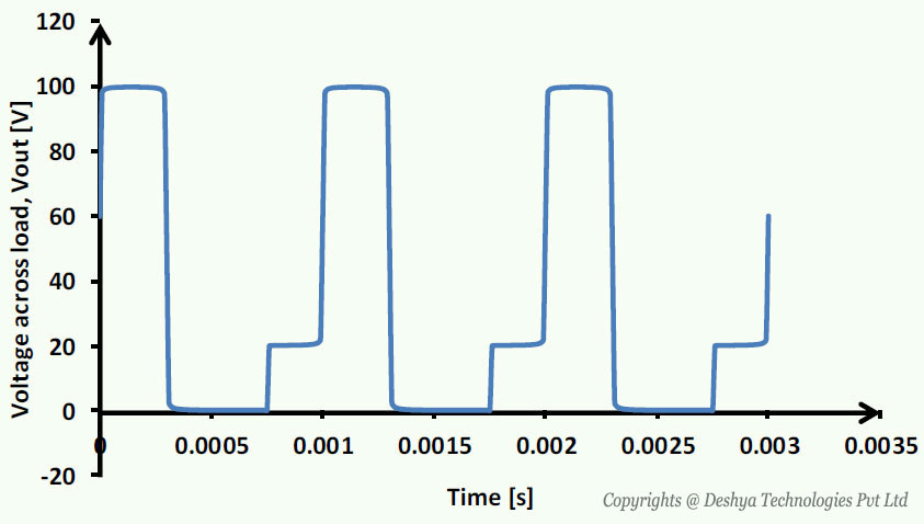
Figure 8.B2.1: Voltage across load for discontinuous mode of conduction..
Figure 8.B2.1: Voltage across load for discontinuous mode of conduction.
The current is given by
 |
(8.B2.9) |
Where
 |
(8.B2.10a) |
 |
(8.B2.10b) |
 |
(8.B2.10c) |
 |
(8.B2.10d) |
The plot of load current using equation 8.B2.9
is shown in figure 8.B2.2 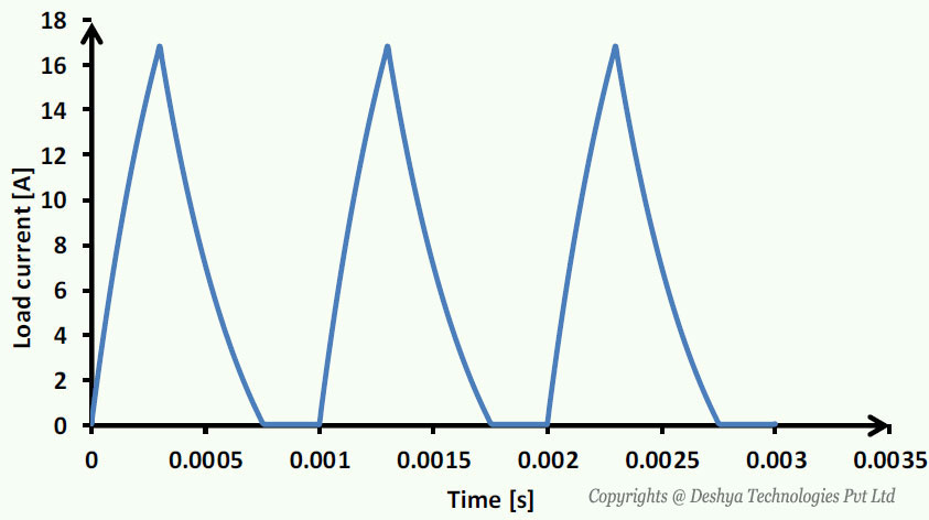
Figure 8.B2.2: Load current for discontinuous mode of conduction..
Figure 8.B2.2: Load current for discontinuous mode of conduction.
8.5: The Buck Converter with R Load and Filter
The output voltage and current of the converter contain harmonics due to the switching action. In order to remove the harmonics LC filters are used. The circuit diagram of the buck converter with LC filter is shown in figure 8.11 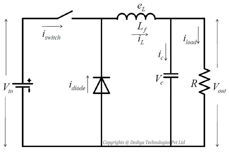
Figure 8.11: Buck converter with L-C filter.. There are two modes of operation as explained in the previous section.
The voltage drop across the inductor in mode 1 is
 |
(8.47) |
where iL is the current through the inductor Lf
iswitch is the current through the switch
The switching frequency of the converter is very high and hence, iL changes linearly. Thus, equation 8.47 
can be written as
 |
(8.48) |
where T1 is the duration for which the switch S remains on
T is the switching time period
Figure 8.11: Buck converter with L-C filter.
Hence, the current ripple ∆iL is given by
 |
(8.49) |
When the switch S is turned off, the current through the filter inductor decreases and the current through the switch S is zero. The voltage equation is
 |
(8.50) |
where idiode is the current through the diode D
Due to high switching frequency, the equation 8.50
can be written as
 |
(8.51) |
where T2 is the duration in which switch S remains off the diode D conducts. Neglecting the very small current in the capacitor Cf, it can be seen that (iload = iswitch) for time duration in which switch S conducts and (iload = idiode) for the time duration in which the diode D conducts.
The current ripple obtained from equation 8.30
is
 |
(8.52) |
The voltage and current waveforms are shown in figure 8.12 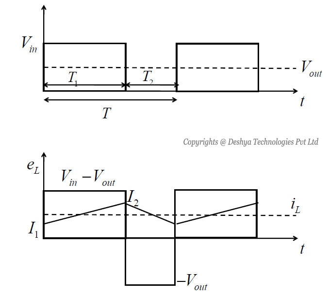
Figure 8.12: The voltage and current through the inductor in a buck conveter with L-C filter..
Figure 8.12: The voltage and current through the inductor in a buck conveter with L-C filter.
From equation 8.49
and equation 8.52
the following relation is obtained for the current ripple
 |
(8.53) |
Hence, from equation 8.53
the relation between input and output voltage is obtained as
 |
(8.54) |
If the converter is assumed to be lossless, then
 |
(8.55) |
The switching period T can be expressed as
 |
(8.56) |
From equation 8.56
the current ripple is given by
 |
(8.57) |
Substituting the value of Vo from equation 8.54
into equation 8.57
gives
 |
(8.58) |
Using the Kirchhoff’s current law, the inductor current is expressed as (see figure 8.11
Figure 8.11: Buck converter with L-C filter.)
 |
(8.59) |
If the ripple in load current (iload) is assumed to be small and negligible, then
 |
(8.60) |
The average capacitor current, which flows into it for (T1/2 + T2/2 = T/2) is
 |
(8.61) |
The capacitor voltage is given by
 |
(8.62) |
The peak-to-peak ripple voltage of the capacitor is
 |
(8.63) |
Substituting the value of ∆IL from equation 8.52
into equation 8.2
gives
 |
(8.64) |
Boundary between Continuous and Discontinuous Conduction
The inductor (iL ) and the voltage drop across the inductor (eL ) are shown in figure 8.13 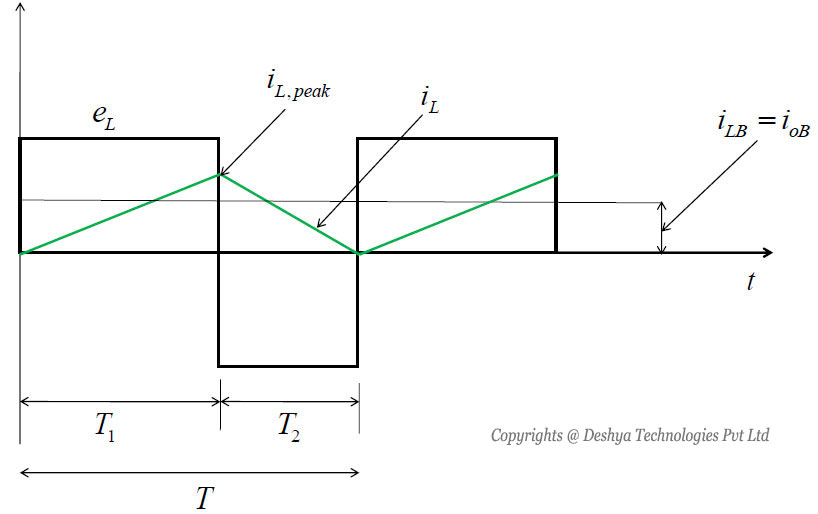
Figure 8.13: The inductor voltage and current waveforms for discontinuous operation..
Figure 8.13: The inductor voltage and current waveforms for discontinuous operation.
Being at the boundary between the continuous and the discontinuous mode, the inductor current iL goes to zero at the end of the off period. At this boundary, the average inductor current is (B referes to the boundary)
 |
(8.65) |
Hence, during an operating condition, if the average output current (IL ) becomes less than ILB, then IL will become discontinuous.
Discontinuous Conduction Mode with Constant Input Voltage Vin
In applications such as speed control of DC motors, the input voltage (Vin) remains constant and the output voltage (Vout) is controlled by varying the duty ratio D. Since Vout = DVin, the average inductor current at the edge of continuous conduction mode is obtained from equation 8.65
as
 |
(8.66) |
In figure 8.14 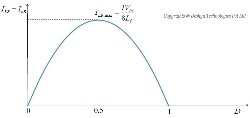
Figure 8.14: General configuration of buck converter. the plot of ILB as a function of D, keeping all other parameters constant, is shown. The output current required for a continuous conduction mode is maximum at D = 0.5 and by substituting this value of duty ratio in equation 8.66
the maximum current (ILB, max) is obtained as
Figure 8.14: Current versus duty ratio keeping input voltage constant.
 |
(8.67) |
From equation 8.66
and equation 8.67
, the relation between ILB and ILB,max is obtained as
 |
(8.68) |
To understand the ratio of output voltage to input voltage (Vout/Vin) in the discontinuous mode, it is assumed that initially the converter is operating at the edge of the continuous conduction (figure 8.13
Figure 8.13: General configuration of buck converter.), for given values of T, L, Vd and D. Keeping these parameters constant, if the load power is decreased (i.e., the load resistance is increased), then the average inductor current will decrease. As is shown in figure 8.15 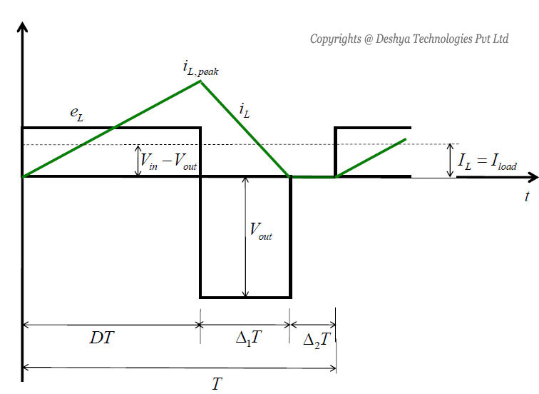
Figure 8.15: Load current and voltage in a buck converter with L-C fileter in discontinuous operation is buck converter., this dictates a higher value of Vo than before and results in a discontinuous inductor current
Figure 8.15: Load current and voltage in a buck converter with L-C filter in discontinuous operation is buck converter.
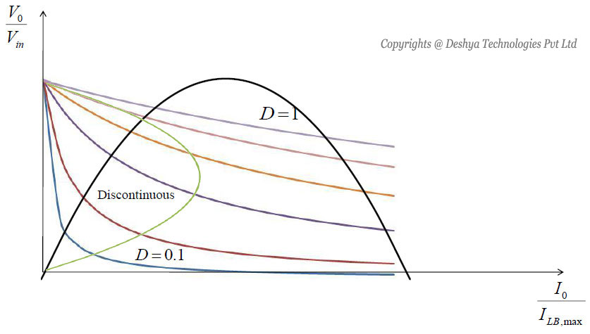
Figure 8.16: Buck converter characteristics for constant input current.
In the time interval ∆2T the current in the inductor Lf is zero and the power to the load resistance is supplied by the filter capacitor alone. The inductor voltage eL during this time interval is zero. The integral of the inductor voltage over one time period is zero and in this case is given by
 |
(8.69) |
In the interval 0 ≤ t ≤ ∆1Ts (figure 8.15
Figure 8.15: Load current and voltage in a buck converter with L-C fileter in discontinuous operation is buck converter.) the current ripple in Lf is
 |
(8.70) |
From figure 8.15
Figure 8.15: General configuration of buck converter. it can be seen that
 (since the current falls) |
(8.71) |
 |
(8.72) |
Substituting the values of ∆iL and eL from equation 8.71
and equation 8.72
into equation 8.70
gives
 |
(8.73) |
 |
(8.74) |
Hence,
 |
(8.75) |
From equation 8.68
and equation 8.74
the ratio Vout / Vin is obtained as
 |
(8.76) |
In figure 8.16
Figure 8.16: Buck converter characteristics for constant input current. the step down characteristics in continuous and discontinuous modes of operation is shown. In this figure the voltage ratio (Vo / Vin) is plotted as a function of Io / ILB, max for various duty ratios using equation 8.55
and equation 8.76
. The boundary between the continuous and the discontinuous mode, shown by dashed line in figure 8.16
Figure 8.16: Buck converter characteristics for constant input current., is obtained using equation 8.54
and equation 8.70
.
Discontinuous-Conduction Mode with Constant Vo
In some applications such as regulated DC power supplies, Vin may vary but Vo is kept constant by adjusting the duty ratio. From equation 8.66
the average inductor current at the boundary of continuous conduction is obtained as
 |
(8.77) |
From equation 8.77
it can be seen that, for a given value of Vo the maximum value of ILB occurs at D = 0 and is given by
 |
(8.78) |
From equation 8.77
and equation 8.78
the relation between ILB and ILB, max is
 |
(8.79) |
From equation 8.74
, the output current is obtained as
 |
(8.80) |
Solving the equation 8.80
for ∆1 and substituting its value in equation 8.69
gives
 |
(8.81) |
8.6: Conclusion:
In this chapter the analysis of DC-DC buck converter was presented. The Fourier series analysis of the output voltage and load current for continuous and discontinuous mode of operation was also presented in this chapter.
The key points of this chapter are:
- When the DC-DC converter feed a resistive load, the current is discontinuous.
- An inductive load can make the load current continuous.
- The critical value of inductance that is required for continuous current depends on the load to e.m.f. ratio.
- The load current ripple becomes maximum for a duty ratio of 0.5.